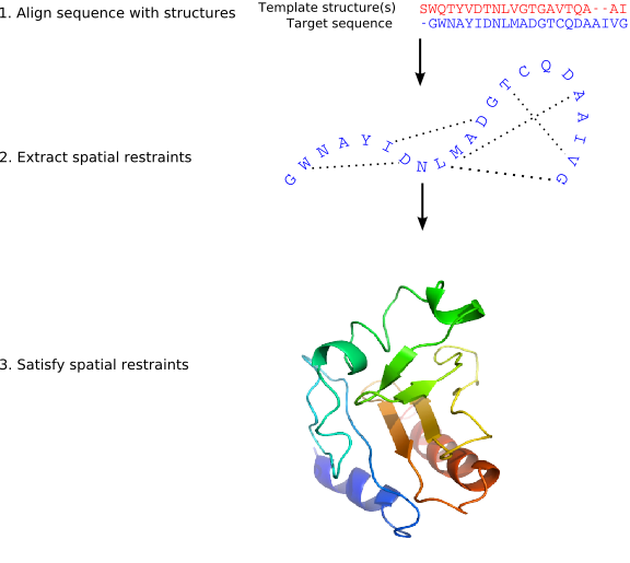
MODELLER implements an automated approach to comparative
protein structure modeling by satisfaction of spatial restraints
(Figure 1.1) [Š
ali & Blundell, 1993]. The method and its
applications to biological problems are described in detail
in references listed in Section 1.2. Briefly,
the core modeling procedure begins with an alignment of the sequence to be
modeled (target) with related known 3D structures (templates). This
alignment is usually the input to the program. The output is a 3D
model for the target sequence containing all mainchain and sidechain
non-hydrogen atoms. Given an alignment, the model is obtained without
any user intervention. First, many distance and dihedral angle
restraints on the target sequence are calculated from its alignment with
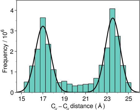
template 3D structures (Figure 1.2). The form of these
restraints was obtained from a statistical analysis of the
relationships between many pairs of homologous structures. This
analysis relied on a database of 105 family alignments that included
416 proteins with known 3D structure [Š
ali & Overington, 1994]. By scanning the
database, tables quantifying various correlations were obtained, such
as the correlations between two equivalent
![]() -
-
![]() distances,
or between equivalent mainchain dihedral angles from two
related proteins. These relationships were expressed as conditional
probability density functions (pdf's) and can be used directly as
spatial restraints. For example, probabilities for different values of
the mainchain dihedral angles are calculated from the type of a
residue considered, from mainchain conformation of an equivalent
residue, and from sequence similarity between the two proteins.
Another example is the pdf for a certain
distances,
or between equivalent mainchain dihedral angles from two
related proteins. These relationships were expressed as conditional
probability density functions (pdf's) and can be used directly as
spatial restraints. For example, probabilities for different values of
the mainchain dihedral angles are calculated from the type of a
residue considered, from mainchain conformation of an equivalent
residue, and from sequence similarity between the two proteins.
Another example is the pdf for a certain
![]() -
-
![]() distance
given equivalent distances in two related protein structures
(Figure 1.2). An important feature of the method is that
the spatial restraints are obtained empirically, from a database of
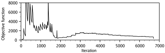
protein structure alignments. Next, the spatial restraints and
CHARMM energy terms enforcing proper stereochemistry
[MacKerell et al., 1998] are combined into an objective function. Finally,
the model is obtained by optimizing the objective function in
Cartesian space. The optimization is carried out by the use of the
variable target function method [Braun & Gõ, 1985] employing methods of
conjugate gradients and molecular dynamics with simulated annealing
(Figure 1.3). Several slightly different models can be
calculated by varying the initial structure. The variability among
these models can be used to estimate the errors in the corresponding
regions of the fold.
distance
given equivalent distances in two related protein structures
(Figure 1.2). An important feature of the method is that
the spatial restraints are obtained empirically, from a database of
protein structure alignments. Next, the spatial restraints and
CHARMM energy terms enforcing proper stereochemistry
[MacKerell et al., 1998] are combined into an objective function. Finally,
the model is obtained by optimizing the objective function in
Cartesian space. The optimization is carried out by the use of the
variable target function method [Braun & Gõ, 1985] employing methods of
conjugate gradients and molecular dynamics with simulated annealing
(Figure 1.3). Several slightly different models can be
calculated by varying the initial structure. The variability among
these models can be used to estimate the errors in the corresponding
regions of the fold.
There are additional specialized modeling protocols, such as that for the modeling of loops (Section 2.3).
|
|
|